Introduction

Most statistical analyses can be written in the form of a simple model.
For example, a linear regression model can be expressed as:

Y = β₀ + β₁X + ε

Here, Y is the outcome, X is a predictor, and ε represents the random error or unexplained variation.

What constant variance really means

The homogeneity of variance assumption concerns the behaviour of the error term ε.

Specifically, the model assumes:

Var(ε | X) = σ²

This says that the variability of the errors is the same for all values of the predictor.
In other words, the spread of the data around the regression line does not systematically increase or decrease as X changes.

This is why the assumption is often called constant variance or homoscedasticity.

Why we assume constant variance

Linear regression and many related methods use a single estimate of variability, σ², to quantify uncertainty.

If the variance truly is constant, this single number accurately reflects how noisy the data are across the entire range of the predictor.

If variance changes with X, this single estimate becomes misleading.
As a result, standard errors, confidence intervals, and p values may no longer be reliable.

How the assumption breaks down

In practice, variance often depends on the level of the outcome or predictor.

Common patterns include:

• Greater variability at higher values of the outcome
• Less variability near natural boundaries such as zero
• Increasing measurement error as values become larger

These situations lead to heteroscedasticity, where:

Var(ε | X) ≠ σ²

How to see it in your data

The simplest way to assess constant variance is to plot residuals against fitted values.

If the assumption holds, residuals form a roughly even band around zero.

If the band fans out or narrows, variance is not constant.

Formal tests such as Levene’s test or the Breusch Pagan test can be used, but visual diagnostics should always come first.

Examples of residual plots

Residual plots provide the most direct way to assess the constant variance assumption.
They show whether the spread of the errors remains stable across the range of fitted values.

Residual plot indicating homoscedasticity

In a well behaved model, residuals are scattered randomly around zero with a roughly constant vertical spread.
There is no visible pattern, and the width of the cloud does not change as fitted values increase.

This pattern is consistent with the assumption:

Var(ε | X) = σ²

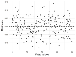Figure 1. Residuals versus fitted values showing approximately constant variance.

Residual plots indicating violation of constant variance

Violations of the homogeneity of variance assumption are usually easy to recognise once you know what to look for.

Funnel or fan shaped pattern

Residuals become progressively more spread out or more tightly clustered as fitted values increase.

This indicates that variance changes with the level of the outcome.

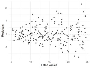
Figure 2. Residual plot showing increasing variance with fitted values.

Unequal spread across groups

When residuals are plotted by group, one group may show much greater variability than others.

This commonly occurs in group comparison studies.

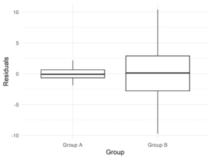
Figure 3. Residuals by group showing unequal variances.

These patterns indicate heteroscedasticity and suggest that standard errors from a classical linear model may be unreliable.

What to do if variance is not constant

A violation of constant variance does not mean the model is useless.
It means the uncertainty needs to be handled differently.

• Use robust standard errors that allow variance to change
• Transform the outcome to stabilise variability
• Use weighted regression when variance structure is known

These approaches allow the model to remain interpretable while restoring valid inference.

Summary

Homogeneity of variance is an assumption about the error term in a statistical model.
It requires that variability around the model is stable across predictors.
When this assumption fails, inference based on standard errors must be adjusted rather than ignored.